MLJ中线性模型在回归预测中的简单使用

开始之前
数据准备
模型介绍
添加特征
最后说明

开始之前

我想向大家介绍一下一些线性模型的用法，以及他们对数据的拟合程度
在我开始学习 MLJ 时，我对他们的拟合能力有所怀疑，经常遇到欠拟合的情况，经过一次简单的测试后，才慢慢了解如何使用模型，处理特征
这里将这个测试介绍给各位

数据准备

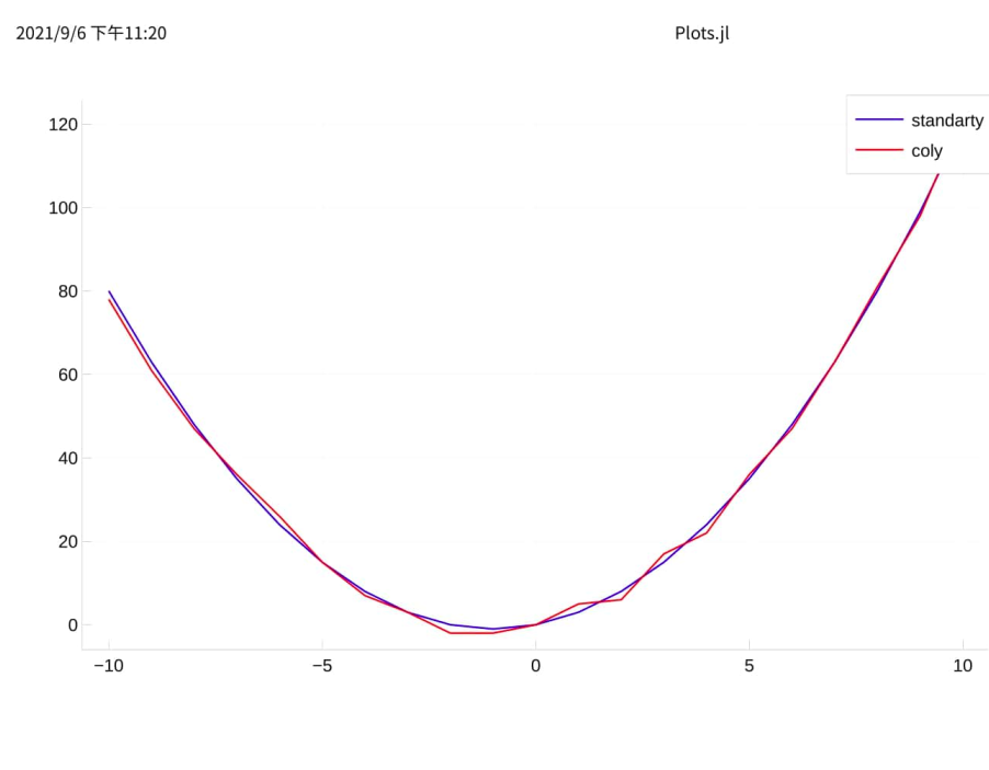
我们模拟对函数 f(x) = x² + 2x 的拟合，在理想的预测结果 standardy 上加上一点噪音，形成训练用测试结果 coly
接下来依次定义

f(x)
standardy
coly

f(x) = x^2 + 2x
colx = DataFrame(x1=-10:10)
coly = f.(colx.x1) + rand(-2:2, length(colx.x1))
standardy = f.(colx.x1)

再绘制下图像

plot(colx.x1, standardy, label="standarty", color=:blue)
plot!(colx.x1, coly, label="coly", color=:red)

模型介绍

拟合数据我们使用 Ridge 回归，他在损失函数上添加了 L2 正则化

\begin{array}{cl} {\min \limits_{w, b}} & {\dfrac{1}{n}\sum_{i = 1}^n (w^{\top} x_i + b - y_i)^2} \\ {\text{s.t.}} &{\|w\|_2^2 \le t} \end{array}

\tag{6}
在 MLJLinearModels 中，RidgeRegressor 为

Ridge regression model with objective function

其中参数有

lambda (Real): strength of the L2 regularisation.
fit_intercept (Bool): whether to fit the intercept or not.
penalize_intercept (Bool): whether to penalize the intercept.
solver: type of solver to use (if nothing the default is used). The solver is Cholesky by default but can be Conjugate-Gradient as well. See ?Analytical for more information.

详细介绍以下 fit_intercept 和 penalize_intercept ，去 Slack 问了以下，大致可以理解为

fit_intercept 在假设函数上是否添加偏差(bias)
penalize_intercept 是否惩罚偏差，修改其数值

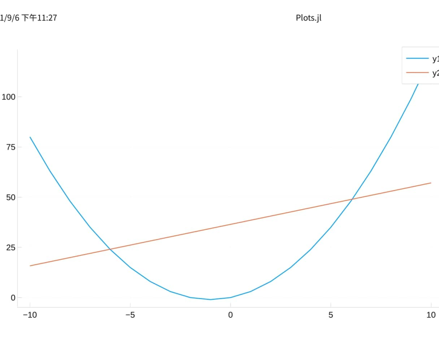
接下来模型训练，直接调优得到最优模型，得到输出结果

using MLJLinearModels, StableRNGs
rng = StableRNG(1234)

ridge = RidgeRegressor()
r_lambda = range(ridge, :lambda, lower = 0.01, upper = 10, scale=:linear)
tuning = Grid(resolution = 20, rng=rng)
resampling = CV(nfolds = 6, rng=rng)
self_tuning_model = TunedModel(model = ridge,
                               range = r_lambda,
                               tuning = tuning,
                               resampling = resampling,
                               measure = rms
                               )
self_tuning_mach = machine(self_tuning_model, colx, coly)
fit!(self_tuning_mach)
best_model = fitted_params(self_tuning_mach).best_model
best_mach = machine(best_model, colx, coly)
fit!(best_mach)
outputy = predict(best_mach, colx)

然后我们通过图像查看拟合程度

plot(colx.x1, standardy, label="standardy", color=:blue)
plot!(colx.x1, outputy, label="outputy", color=:red)

可以看到，欠拟合了

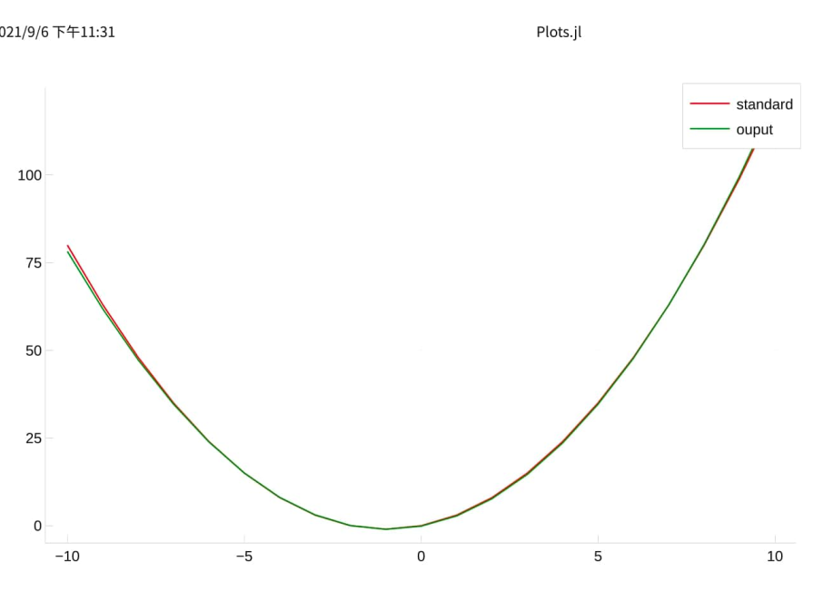
添加特征

应对欠拟合的情况我们可以通过添加特征来解决
回到上面的问题，由于 f(x) = x² + 2x ，提供的数据中只有 x1=x 一个特征，我们尝试再添加一个特征 x2=x²

let g(x) = x^2
  colx.x2 = g.(colx.x1)
  self_tuning_machine = machine(self_tuning_model, colx, coly)
  fit!(self_tuning_machine)
  best_model = fitted_params(self_tuning_mach).best_model
  best_mach = machine(best_model, colx, coly)
  fit!(best_mach)
  outputy = predict(best_mach, colx)

  plot(colx.x1, standardy, label="standardy", color=:blue)
  plot!(colx.x1, outputy, label="output", color=:red) |> display
end

可以看到，挺完美
那我们再添加一个特征 x3=x³

let g(x) = x^3
  colx.x3 = g.(colx.x1)
  self_tuning_machine = machine(self_tuning_model, colx, coly)
  fit!(self_tuning_machine)
  best_model = fitted_params(self_tuning_mach).best_model
  best_mach = machine(best_model, colx, coly)
  fit!(best_mach)
  outputy = predict(best_mach, colx)

  plot(colx.x1, standardy, color=:blue, label="standard")
  plot!(colx.x1, outputY, color=:red, label="ouputy") |> display
end

最后说明

这次测试没有使用训练集和测试集，相当简陋，只是作为实验

MLJ中 线性模型 在回归预测中的简单使用